Personalize your customer journey with the RFM segmentation, Part I
A statistical approach
By Housni Hassani in Marketing Business Analytics Customer Insights Machine Learning
April 1, 2022
This is the Part I of a two-part series named: “Personalise your customer Journey With RFM segmentation”.
An online retail wants to better understand their customers in order to perform targeted marketing actions. In others words, the eRetail business wants to know which customers are active and which ones are moving from active to inactive. Knowing that will help the online retail to create targeted marketing to keep customers active. To solve this business challenge, we will use a grouping technique called customer segmentation, and group customers by their purchase behaviors.
Customer segmentation is the process of dividing a group customers into subgroups using specific elements e.g. demographics, geographic, psychographic, etc. There are multitude of way to perform a customer segmentation. In this two-part series, we will focus on a popular, easy to use and effective segmentation method called RFM segmentation
This topic will be a two-part series:
- Part 1: This article will focus on RFM segmentation using a statistical method (hierarchical clustering).
- Part 2: The next article in the series will focus on RFM segmentation using managerial approach
How should we split my customers?
There are infinite criteria that can be used to segment customers . However, there is a popular, an effective, and an easy-to-use segmentation method named RFM segmentation that use customers purchase behavior to group customer. In the RFM segmentation:
- R stands for Recency. When was the last time the customer - purchased something?
- F stand for Frequency. What is the number of total purchases made by the customer?
- M stands for Monetary. What is the average amount spent when purchasing something?
It’s an excellent tool for marketers to target specific customers with communications and actions that are relevant for their behavior. Most specifically, it can help companies to manage wisely their budget,to increase revenue and profit by increasing sales, to better understand their customers, to gain competitive advantage against competitors, etc.
How can we perform the RFM segmentation in R ?
About the data
In this work, we will use the online store data set from the UCL repository available. Here. The data set contains all the transactions occurring for a UK-based and registered, non-store online retail between 01/12/2009 and 09/12/2011.The company mainly sells unique all-occasion gift-ware. Many customers of the company are wholesalers."
Step 1: Installing the relevant pacakages and calling their libraries
The pacman package is used as package manager. It combines functionality of base library related functions into intuitively named function.
# install and Load the relevant packages

if(!require("pacman")) install.packages("pacman")
p_load(readxl,tidyverse,factoextra,parameters,gridExtra,kableExtra,NbClust)
Step 2: Data Overview
# Charge the data set:
o.data <- read.csv("https://raw.githubusercontent.com/hhousni/rfm_analysis/main/Online%20Retail.csv")

# Quick look on the structure of the data set:
str(o.data)
## 'data.frame':	541909 obs. of  8 variables:
##  $ ï..InvoiceNo: chr  "536365" "536365" "536365" "536365" ...
##  $ StockCode   : chr  "85123A" "71053" "84406B" "84029G" ...
##  $ Description : chr  "WHITE HANGING HEART T-LIGHT HOLDER" "WHITE METAL LANTERN" "CREAM CUPID HEARTS COAT HANGER" "KNITTED UNION FLAG HOT WATER BOTTLE" ...
##  $ Quantity    : int  6 6 8 6 6 2 6 6 6 32 ...
##  $ InvoiceDate : chr  "1/12/2010 8:26" "1/12/2010 8:26" "1/12/2010 8:26" "1/12/2010 8:26" ...
##  $ UnitPrice   : num  2.55 3.39 2.75 3.39 3.39 7.65 4.25 1.85 1.85 1.69 ...
##  $ CustomerID  : int  17850 17850 17850 17850 17850 17850 17850 17850 17850 13047 ...
##  $ Country     : chr  "United Kingdom" "United Kingdom" "United Kingdom" "United Kingdom" ...
The data set contains 9 variables :
- InvoiceNo: Invoice number. Nominal. A 6-digit integral number uniquely assigned to each transaction. If this code starts with the letter ‘c’, it indicates a cancellation.
- StockCode: Product (item) code. Nominal. A 5-digit integral number uniquely assigned to each distinct product.
- Description: Product (item) name. Nominal.
- Quantity: The quantities of each product (item) per transaction. Numeric.
- InvoiceDate: Invice date and time. Numeric. The day and time when a transaction was generated.
- UnitPrice: Unit price. Numeric. Product price per unit in sterling
- CustomerID: Customer number. Nominal. A 5-digit integral number uniquely assigned to each customer.
- Country: Country name. Nominal. The name of the country where a customer resides
Step 3: Data Preparation and Exploration
Data Prep
As mentioned earlier, to perform the RFM segmentation, we need to determine for each customer it recency, frequency and, monetary values. As we can see, the data set doesn’t contain these variables. They need to be calculated. The first step of the data prep is to select the relevant variables necessary to determine the RFM indicators.
# Select the relevant variables:
dataprep0 <- o.data %>%
  select(CustomerID, Quantity, UnitPrice, InvoiceDate) %>%
  mutate(InvoiceDate=as.Date(InvoiceDate, "%d/%m/%Y")) %>%
  filter(InvoiceDate >= "2011-01-01" & InvoiceDate <= "2011-12-31")

summary(dataprep0)
##    CustomerID        Quantity           UnitPrice          InvoiceDate
##  Min.   :12346    Min.   :-80995.00   Min.   :-11062.06   Min.   :2011-01-04
##  1st Qu.:13923    1st Qu.:     1.00   1st Qu.:     1.25   1st Qu.:2011-04-21
##  Median :15116    Median :     3.00   Median :     2.08   Median :2011-08-05
##  Mean   :15271    Mean   :     9.68   Mean   :     4.48   Mean   :2011-07-21
##  3rd Qu.:16770    3rd Qu.:    10.00   3rd Qu.:     4.13   3rd Qu.:2011-10-25
##  Max.   :18287    Max.   : 80995.00   Max.   : 38970.00   Max.   :2011-12-09
##  NA's   :119449
The table above shows negative values in the quantity and the UnitPrice variables, we will need to remove them. But before let check the presence of missing value in the data set.
# Look for missing values:
sapply(dataprep0, function (x) sum(is.na(x)))
##  CustomerID    Quantity   UnitPrice InvoiceDate
##      119449           0           0           0
As we can see, CustommerID contains 119449. CustomerID is an important variable to interpret the results and to implement the post hoc Marketing strategic actions. Without it the analyse is useless. It’s necessary to remove the customers without ID to proceed.
# remove the missing values and the negative value in the quantity and UnitPrice
dataprep1 <- dataprep0 %>%
  drop_na(CustomerID) %>%
  filter(Quantity > 0, UnitPrice > 0 )
Create rencey, frequency and, monetary indicators.
# Create the relevant Monetary
dataprep2 <- dataprep1  %>%
  mutate (purchase_amount = (Quantity * UnitPrice)) %>%
  arrange(CustomerID) %>%
  group_by(CustomerID,InvoiceDate) %>%
  summarise(Sales = sum(purchase_amount))

# Show the lastest date in the data set. This value is going to be used to calculate recency
print (max(dataprep2$InvoiceDate))
## [1] "2011-12-09"
# Create recency variable, we consider this study to be conducted one day after the last purchase in the data set. Create the Monetary and frequency.
f.dataprep <- dataprep2 %>%
  mutate(datediff =as.numeric(as.Date("2011-12-10") - InvoiceDate)) %>%
  group_by(CustomerID) %>%
  summarise(monetary  = mean(Sales),
            recency   = min(datediff),
            frequency = n())

# Store the Customer ID variable to use it later
customerID <- f.dataprep$CustomerID

# Select the data with only the marketing indicators
rfm.data <- f.dataprep [,c("monetary", "recency", "frequency")]
Exploratory Analysis
summary(rfm.data)
##     monetary           recency         frequency
##  Min.   :    3.45   Min.   :  1.00   Min.   :  1.000
##  1st Qu.:  186.96   1st Qu.: 18.00   1st Qu.:  1.000
##  Median :  307.40   Median : 48.00   Median :  2.000
##  Mean   :  463.02   Mean   : 85.35   Mean   :  3.687
##  3rd Qu.:  456.82   3rd Qu.:129.00   3rd Qu.:  4.000
##  Max.   :84236.25   Max.   :340.00   Max.   :122.000
The online store’s customers have spent on average £463, with a minimum amount of £3.45 and a maximum amount of £84236. They purchase in average 3.6 times with a minimum of 1 time and a maximum of 122 times. The average customer last purchases were 85 days ago, some of them did they last purchase a day prior to the study and other 339 days.
Both descriptive statistics and histograms shows that the data set is to be skewed to the right.It means the most data are on the left but a few larger values are on the right. The few larger values bring the mean upwards but don’t really affect the median. To respond to skewness towards large value of amount variables and the different scale, we are going to do a log transformation of the variables, standardize and scale the data set.
logRfm.data <- rfm.data %>%
  mutate(monetary  = log(monetary),
         recency   = log(recency),
         frequency = log (frequency))

scaledata <- as.data.frame(scale(logRfm.data))
Application
Before running hierarchical segmentation let’s see how the ascending hierarchical clustering works:
- Every point is one cluster.
- Calculate the distance between each point/cluster
- Merge 2 points/clusters that are closest to each other based on the distance.
- Recalculate the distance between the new and/or old clusters
- Merge 2 clusters that are closest to each other based on the distance.
- Repeat 1,2,3 and, 4 until all cluster are merged into one single cluster including all points.
There are 5 main methods to measure the distance between cluster before merging them. In this analysis, we use the ward’s criterion. minimizes the total within-cluster variance and find the pair of clusters that leads to minimum increase in total within-cluster variance after merging.
Choosing the Optimal Number of Clusters
Different methods have been proposed for determining the optimal number of clusters among them, there are:
- The Elbow Method
- The Gap Statistic
- The Silhouette Method
- The Sum of Squares Method
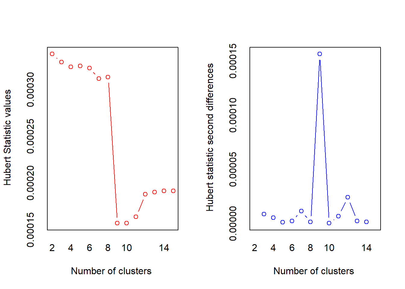
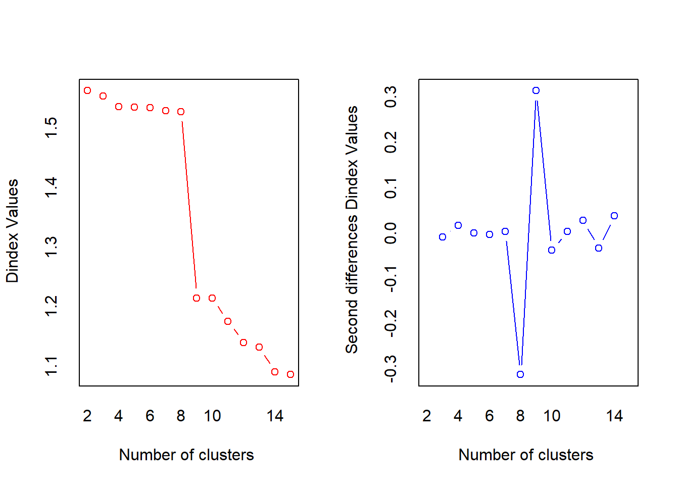
Each on has they pros and cons, benefits and limitation. However, there is the NbClust package performs the clustering and compute a maximum of 30 indices and propose to users the best clustering scheme from the different results obtained by varying all combinations of number of clusters, distance measures, and clustering methods.
set.seed(12345)

optimalCluster <- NbClust(scaledata, method = "average")

## *** : The Hubert index is a graphical method of determining the number of clusters.
##                 In the plot of Hubert index, we seek a significant knee that corresponds to a
##                 significant increase of the value of the measure i.e the significant peak in Hubert
##                 index second differences plot.
##

## *** : The D index is a graphical method of determining the number of clusters.
##                 In the plot of D index, we seek a significant knee (the significant peak in Dindex
##                 second differences plot) that corresponds to a significant increase of the value of
##                 the measure.
##
## *******************************************************************
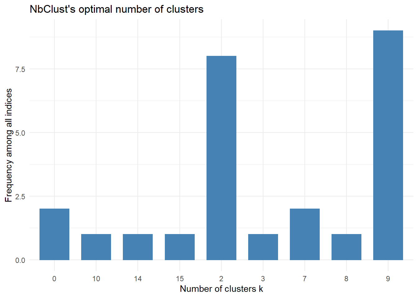
## * Among all indices:
## * 8 proposed 2 as the best number of clusters
## * 1 proposed 3 as the best number of clusters
## * 2 proposed 7 as the best number of clusters
## * 1 proposed 8 as the best number of clusters
## * 9 proposed 9 as the best number of clusters
## * 1 proposed 10 as the best number of clusters
## * 1 proposed 14 as the best number of clusters
## * 1 proposed 15 as the best number of clusters
##
##                    ***** Conclusion *****
##
## * According to the majority rule, the best number of clusters is  9
##
##
## *******************************************************************
factoextra::fviz_nbclust(optimalCluster) + theme_minimal() + ggtitle("NbClust's optimal number of clusters")
## Among all indices:
## ===================
## * 2 proposed  0 as the best number of clusters
## * 8 proposed  2 as the best number of clusters
## * 1 proposed  3 as the best number of clusters
## * 2 proposed  7 as the best number of clusters
## * 1 proposed  8 as the best number of clusters
## * 9 proposed  9 as the best number of clusters
## * 1 proposed  10 as the best number of clusters
## * 1 proposed  14 as the best number of clusters
## * 1 proposed  15 as the best number of clusters
##
## Conclusion
## =========================
## * According to the majority rule, the best number of clusters is  9 .

The NbClust suggested 9 as optimal cluster number
Running The Algorithm
Let now run the hierarchical algorithm.
set.seed(1234)

# Determine the distance in the standardize and scaled data:

d= dist(scaledata)

# perform the hierarchical Segmentation:

hc = hclust(d, method = "ward.D2")

# plot the dendrogram

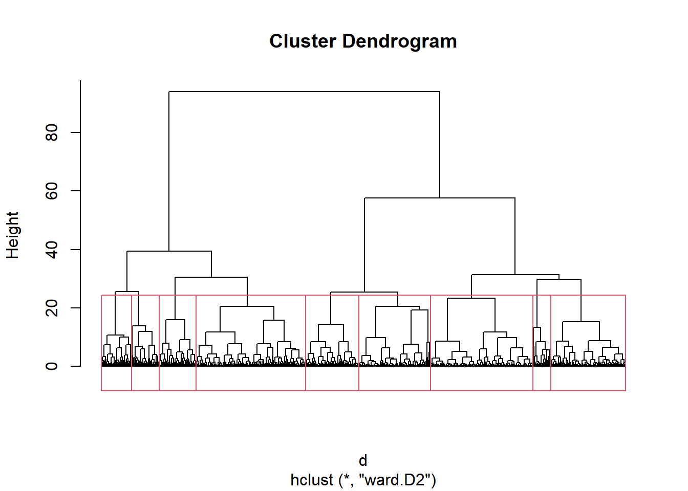
plot (hc, hang = -1, labels = FALSE)
rect.hclust(hc, k = 9)

set.seed(45678)
# Cut the dendrogram with the optimal number of clusters

members = cutree(hc, k=9)

tableMembers <- as.data.frame(table(members))

aggregate <- aggregate(rfm.data , by = list(members), mean)

# Group aggregate value by cluster with number of customer.

avgcluster <- bind_cols(aggregate,tableMembers) %>%
  select ("cluster" = Group.1, monetary, recency, frequency, "nb.customer" = Freq)

avgcluster
##   cluster  monetary    recency frequency nb.customer
## 1       1 3256.2091 141.048611  1.291667         144
## 2       2 1215.0808  15.677273  7.277273         220
## 3       3  469.3522 105.708333  2.840000         600
## 4       4  391.3766 141.178182  1.000000         825
## 5       5  333.7873  27.754545  5.052273         880
## 6       6  127.7780 149.594454  1.031196         577
## 7       7  258.0867   5.422819  2.932886         298
## 8       8  430.1046   5.832653 16.967347         245
## 9       9  146.5755  99.153488  2.718605         430
The results above show for each cluster the monetary, recency and frequency average value and the number of customer within. We can see that:
- The cluster 1 contains 144 customers. In the study’s period, they have spent in average £3256 in 1 purchase time and they have made they last purchase 141 days prior the study.
- The cluster 2 contains 220 customers. In the study’s period, they have spent in average £1215 in 7 purchase time and they have made they last purchase 15 days prior the study
- The cluster 3 contains 600 customers. In the study’s period, they have spent in average £469 in 3 purchase time and they have made they last purchase 105 days prior the study
- etc.
Now let combine the hierarchical results with the customer ID and the clean data set to be able to select all the customer by cluster.
# Put customerID, the clean data set and the results together

customerDataCluster <-cbind(members,customerID,rfm.data)
names(customerDataCluster) <- c("cluster","customerID","monetary","recency","frequency")

# Select for each cluster, it customers

cluster_1 <- customerDataCluster %>%
    filter(members==1)

cluster2 <- customerDataCluster %>%
  filter(members==2)

cluster_3 <- customerDataCluster %>%
    filter(members==3)

cluster_4 <- customerDataCluster %>%
    filter(members==4)

cluster_5 <- customerDataCluster %>%
    filter(members==5)

cluster_6 <- customerDataCluster %>%
    filter(members==6)

cluster_7 <- customerDataCluster %>%
    filter(members==7)

cluster_8 <- customerDataCluster %>%
    filter(members==8)

cluster_9 <- customerDataCluster %>%
    filter(members==9)
Now, we have every cluster and it customers. We can apply for each segment the marketing strategic actions.
Marketing Strategic Actions
The hierarchical segmentation has allowed us to find out that our Data is composed by 9 segments. Below are the characteristics of every segment and some actions that can be taken
| Segment.Name | Cluster.Number | Description | Actions |
|---|---|---|---|
| Champions | Cluster 2 | Spent the most, bought recently, often ordered | Need to be rewarded, Great Ambassador |
| Potential Loyalist | Cluster 8 | Recent Customer, spend a good amount | Upsell higher-value products. Ask for reviews |
| New Customers | Cluster 7 | Bought recently with the lowest frequency | Provide on boarding support, early access, start building relationship |
| Core Customers | Cluster 2 | Standard customers purchased not too long | Limited offers |
| Need attention | Cluster 5 | Core customers with last purchase a month ago | Make limited time offers, personalized recommendations |
| Customers At Risk | Cluster 3 and 9 | Few purchase, Small spending, haven't returned long time ago | Personalise reactivation campaigns, offer renewal and helpful products |
| Lost Customers | Cluster 1, 4 and 6 | Only one purchase long time ago and didn't engage after | Reach out campaign. Otherwise they can be ignored |
Conclusion and Limits
Conclusion
In this exercise, we wanted to perform an RFM segmentation using the statistical approach on an online store data set. We chose the Hierarchical method. The result led us to divide the customer’s data set into 9 segments. We have defined and give few actions that can be taken for each cluster.
Limites
The statistical approach for segmentation is a good tool BUT not every time. Indeed, it’s very useful when we need a one-shot segmentation i.e. when it doesn’t require frequents update. But when the segmentation needs to be updated frequently. It’s a highly costly method. And that is what we’re faced here with the online store dataset. In facts, for an online store, customer data are frequently updated. Customers’ behaviour change frequently: some of them disappear, new customers are acquired, some customers change segment, etc. In this scenario, the statistical approach isn’t the best option. Instead, companies can use a Managerial Segmentation (set of rules) to perform the RFM segmentation. In one next post, we are going to show how to impplement a managerial segmentation in R.